MicroCFD®
Software Tutorial
Below are links to the currently available video tutorials for the 2D & 3D Virtual Wind Tunnel. More tutorial videos will be added in the future, so please check back from time to time. The 2D Virtual Wind Tunnel also has a text tutorial with step by step instructions. Either text tutorial edition (Edu / Pro) can be accessed within the program environment in PDF for printing. If you have any questions, please contact Help.
|
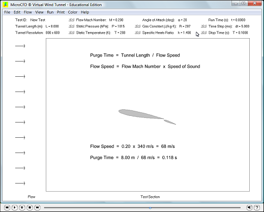
2D Virtual Wind Tunnel Intro - Part 1
|
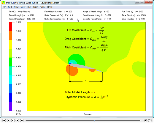
2D Virtual Wind Tunnel Intro - Part 2
|
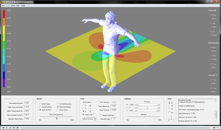
3D Virtual Wind Tunnel Intro